24 Computer Setting for Bioinformatics

Authors

Matin Nuhamunada

Ahmad Ardi

24.1 Introduction

Bioinformatics research requires appropriate hardware and software resources, depending on the type of data and analyses being performed. In this practical session, participants will explore their own computer systems in more detail and learn how to configure them properly to support bioinformatics workflows.

24.2 Computer Specifications

Before starting any analysis, participants should understand the technical specifications of the computer they are using, including:

The Operating System
The system architecture (32-bit / 64-bit)
The type, number of cores, and clock speed of the processor (CPU)
The type and capacity of memory (RAM)
The type and capacity of the graphics card (GPU)
The type and storage capacity of the disk drive (SSD / HDD)

Understanding these specifications helps identify potential computational limitations that may affect data processing and analysis.

24.3 Why UNIX and Scripting?

One of the main goals of this practical session is to introduce participants to the UNIX environment (Linux) and to develop familiarity with scripting. Scripting refers to writing simple command-based instructions that automate repetitive manual tasks.

Although many applications provide user-friendly graphical interfaces, most bioinformatics tools—especially those developed in recent research—are distributed as libraries or Command Line Interface (CLI) programs designed to run within a UNIX environment, often without a Graphical User Interface (GUI) (Welch et al. 2014).

While scripting may not be essential for small-scale or simple analyses, it becomes increasingly important when working with large-scale “omics” datasets and other forms of big data in biological research.

24.4 Tutorial

The following tutorial is adapted from the Data Carpentry lesson “Introduction to the Command Line for Genomics” by the Data Carpentry team, licensed under CC-BY 4.0.

24.4.1 Video Tutorials

Open Setup Video in Google Drive

Open Hands-On Video in Google Drive

Open SSH IP Update Video in Google Drive

24.4.1.0.1 Step-by-Step Screenshot Walkthrough

Visual annotations contributed by: Shiddharta Arya Anggoro Cen

Step 1: Open the Remote Explorer in VS Code and click on the settings gear icon to edit your SSH configuration file.

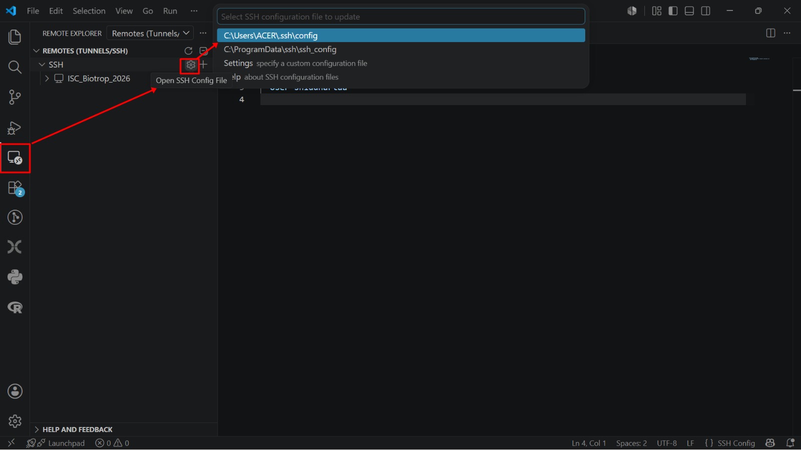
Select SSH Configuration File
Step 2: Open the config file (usually located under ~/.ssh/config or in Windows at C:/Users/username/.ssh/config).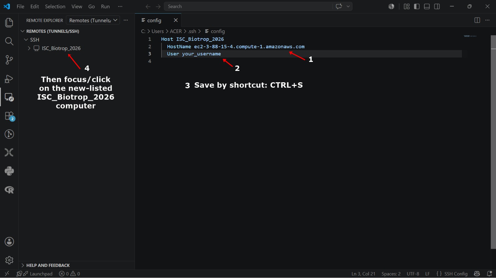

Open config file
Step 3: Update the HostName field with the new IP address provided by your instructor. Save the file.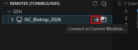

Update HostName IP
Step 4: Right-click the host name in the Remote Explorer sidebar and click Connect to Host in Current Window (or New Window) to log in with the new IP.

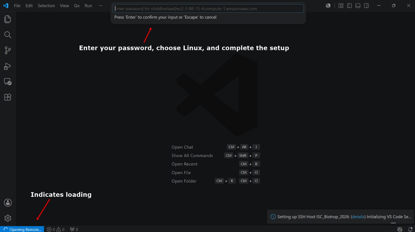
Reconnect to SSH Host
Step 5: Enter the SSH password when prompted at the top of the VS Code window to complete the connection.

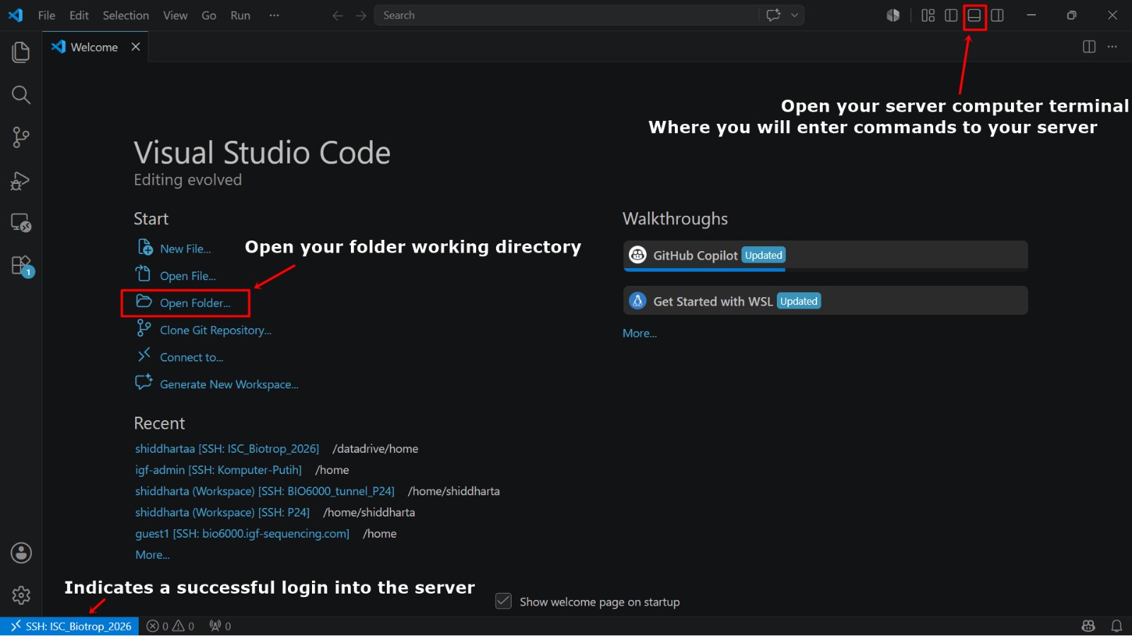
Enter SSH Password
Step 6: Once successfully connected, the bottom-left corner of VS Code will display the active SSH connection status (e.g., SSH: user@ip_address).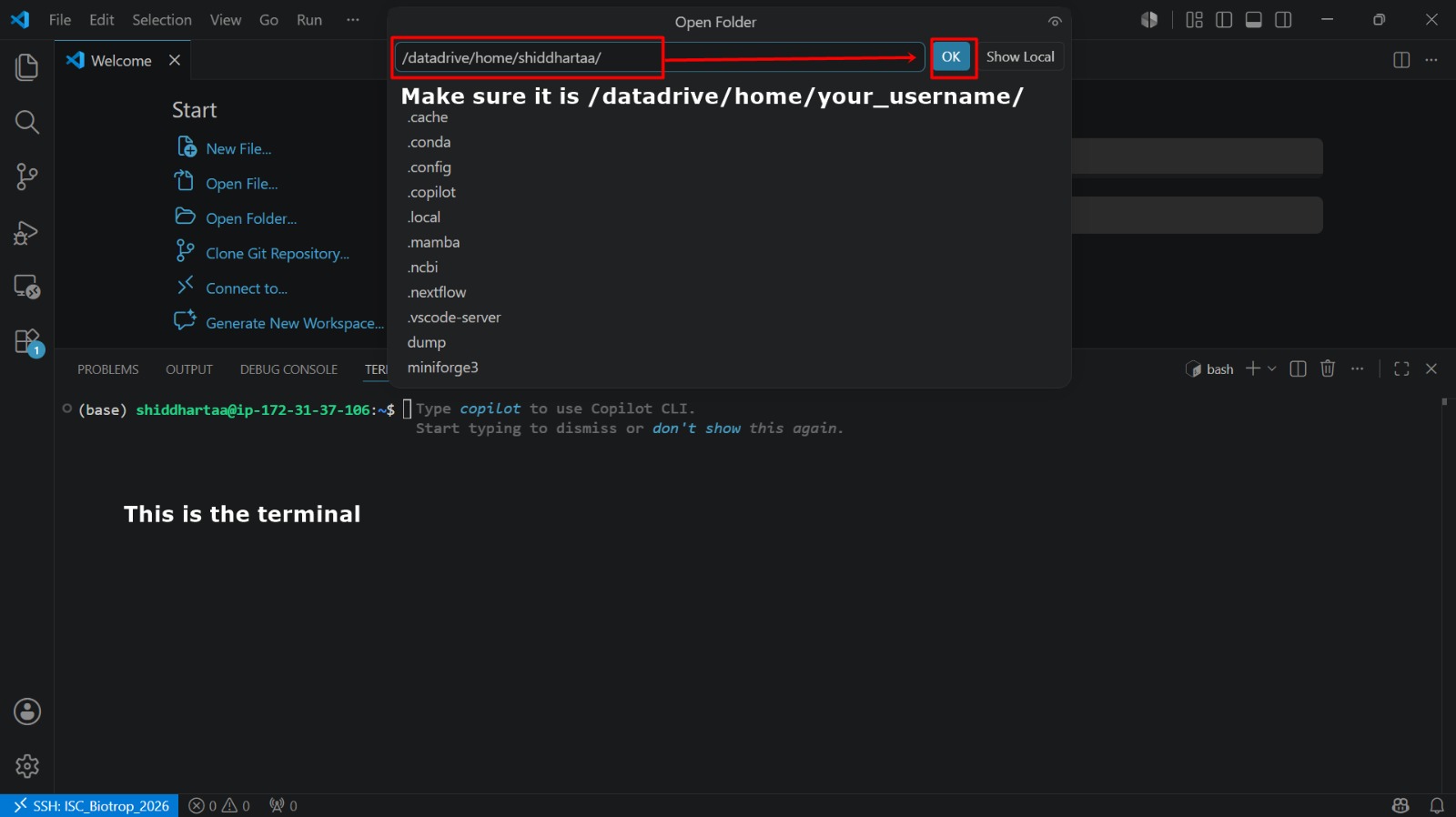

Verify connection status
Step 7: Open a new terminal (Ctrl+Shift+ or Terminal -> New Terminal) to start running commands on the remote Linux environment.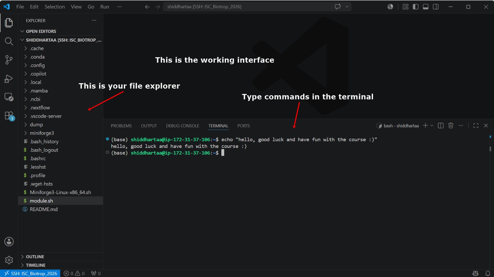

Open terminal and start working

24.4.2 Access the remote server with VS Code

In this tutorial, you will connect to a remote Linux server where the bioinformatics tools and data are already pre-installed. You will access this server using Visual Studio Code (VS Code) with the Remote - SSH extension, which gives you a full-featured editor alongside the terminal — all running on the remote machine.

24.4.2.1 Install VS Code

If you do not already have VS Code installed, download the installer for your operating system from code.visualstudio.com and run it.

24.4.2.2 Install the Remote - SSH Extension

Open VS Code. Click the Extensions icon in the left sidebar (or press Ctrl+Shift+X), search for Remote - SSH, and click Install.

24.4.2.3 Connect to the Remote Server

Your instructor will provide the IP address and password you need to log in.

Open the command palette (Ctrl+Shift+P or Cmd+Shift+P on macOS).
Type Remote-SSH: Connect to Host... and select it.
Enter ssh user@ip_address (replace user and ip_address with the credentials given by your instructor) and press Enter.
When prompted, choose a location to save the host configuration (select the first option, ~/.ssh/config).
A new VS Code window will open. When prompted, enter the password and press Enter.

Once connected, VS Code shows the remote server’s file system in the Explorer sidebar. You are now working directly on the server.

24.4.2.4 Open the Integrated Terminal

Press Ctrl+` (Ctrl + backtick) or go to Terminal → New Terminal in the menu bar. The terminal panel opens at the bottom of the window, already connected to the remote server.

All the shell commands in the following sections should be typed into this terminal panel.

24.4.3 Download tutorial data

First, let’s download the example FASTQ file we will use throughout this tutorial. The file contains real sequencing reads from NCBI’s Sequence Read Archive, but we will only keep the first 250 reads so it is easy to work with.

wget -qO- ftp://ftp.sra.ebi.ac.uk/vol1/fastq/SRR098/SRR098026/SRR098026.fastq.gz | gunzip | head -n 1000 > SRR098026.fastq
ls -lh SRR098026.fastq

The file is about 32 KB in size, making it fast to download and easy to inspect by hand. All the commands in the following sections assume you are in the same directory where you downloaded this file.

24.4.4 Navigate the filesystem

The UNIX command line (BASH / Terminal) is one of the most important working environments in bioinformatics. Let’s start by finding where we are and what files are available.

pwd          # print working directory — shows your current location
ls           # list files and directories
ls -F        # add / to directory names, * to executables
ls -l        # long format: file sizes, permissions, modification dates
mkdir practice && cd practice && cd ..  # create, enter, then leave a directory
cd ~         # return to your home directory

Use the Tab key to auto-complete file and directory names as you type.

24.4.5 Examine files

Bioinformatics data files come in standard formats. Let’s look at a FASTQ file—the standard format for sequencing reads. Each read spans four lines: an identifier, the DNA sequence, a separator (+), and quality scores.

ls *.fastq                              # list all FASTQ files
head -n 4 SRR098026.fastq              # view the first complete read
tail -n 4 SRR098026.fastq              # view the last read
less SRR098026.fastq                   # scroll through the file (press q to quit)
wc -l SRR098026.fastq                  # count total lines in the file

Use head -n 20 or tail -n 20 to see more lines. less lets you browse interactively—use Space to scroll and / to search.

24.4.6 Create, copy, move, remove

Keeping your project organised prevents data loss and confusion.

mkdir backup                             # create a new directory
cp SRR098026.fastq backup/               # copy a file into the directory
mv SRR098026.fastq SRR098026_original.fastq  # rename a file
mv SRR098026_original.fastq SRR098026.fastq  # rename it back
rm unwanted_file.txt                     # delete a file (permanent—use with care)

Always keep a write-protected copy of your raw data:

chmod -w backup/SRR098026.fastq          # remove write permission

24.4.7 Search within files

Real datasets are too large to read by eye. grep searches for patterns inside files without opening them.

grep ACGT SRR098026.fastq               # find lines containing the motif ACGT
grep -c NNNNNNNNNN SRR098026.fastq      # count lines with 10+ unknown bases (Ns)
grep -B1 -A2 NNNNNNNNNN SRR098026.fastq # show full read records around each match

The -c flag gives a count, -B1 shows 1 line before each match, and -A2 shows 2 lines after.

24.4.8 Redirect and pipe

Rather than letting output scroll past your screen, save it to a file or chain commands together.

# Save filtered reads to a new file
grep -B1 -A2 NNNNNNNNNN SRR098026.fastq > bad_reads.txt

# Count the number of lines saved
wc -l bad_reads.txt

# Count matching reads without creating an intermediate file
grep -B1 -A2 NNNNNNNNNN SRR098026.fastq | wc -l

Use > to overwrite a file, >> to append, and | to send output to the next command.

Mini Exercise: How many reads are in your FASTQ file?

Count the total lines: wc -l SRR098026.fastq
Divide by 4 (each read = 4 lines): echo $((1000/4))
Find reads with 10+ unknown bases (Ns):
grep -B1 -A2 NNNNNNNNNN SRR098026.fastq | grep -v '^--' > bad_reads.txt
wc -l bad_reads.txt then divide by 4

This is how you assess sequencing quality before running a real analysis.

24.4.9 Automate with loops

When you have many files, loops let you run the same command on all of them:

for filename in *.fastq; do
    echo "Processing ${filename}"
    head -n 2 ${filename}
done

Use basename to strip file extensions inside a loop:

for filename in *.fastq; do
    name=$(basename ${filename} .fastq)
    echo "${name}"
done

24.4.10 Next steps

This tutorial covered the essential UNIX skills needed for bioinformatics: navigating files, examining data, searching for patterns, and automating repetitive tasks. These skills will serve as a foundation for all subsequent bioinformatics modules in this course.

For a deeper treatment with more exercises and real genomics data, explore the full Data Carpentry lesson:

Data Carpentry — Introduction to the Command Line for Genomics
https://datacarpentry.github.io/shell-genomics/
Source repository: https://github.com/datacarpentry/shell-genomics (CC-BY 4.0)

24.5 Managing Your Environment with Conda

Conda is a package management and environment management tool used to download, install, manage, and remove various software packages and libraries used in programming, including those in computer science and bioinformatics. Conda allows users to manage software dependencies efficiently, ensuring that required tools and libraries are properly installed and compatible with one another.

24.5.1 Why Do We Need a Virtual Environment?

A virtual environment is a named, isolated, working copy of Python or other library that maintains its own files, directories, and paths so that you can work with specific versions of libraries or Python itself without affecting other Python projects. Virtual environments make it easy to cleanly separate different projects and avoid problems with different dependencies and version requirements across components.

Why is this important in bioinformatics? In bioinformatics, different tools often require different versions of Python, specific library versions, and particular dependency configurations. Without isolated environments, installing one package may break another tool due to version conflicts. Virtual environments help prevent these dependency conflicts and ensure reproducibility. They are especially important when you are running multiple analysis pipelines, reproducing published research, sharing workflows with collaborators, and managing long-term research projects.

🔗 Further reading: Conda User Guide: Managing Environments

24.5.2 Installing Conda via Linux / Terminal

When working on a personal computer, you must first install a package manager such as conda or mamba. In this practical, we will install it using the Miniforge distribution.

Miniforge is a lightweight Conda installer that defaults to the community-driven conda-forge channel, making it particularly suitable for scientific and bioinformatics workflows.

Download the installer that matches your system specifications from: Miniforge.

BASE_URL="https://github.com/conda-forge/miniforge/releases/latest/download"
wget "${BASE_URL}/Miniforge3-$(uname)-$(uname -m).sh"

Check that the installer has been successfully downloaded:
```
ls
```
Hint: The downloaded file should have a .sh extension.
Start the installation process:
```
bash Miniforge3-*.sh
```
Follow the on-screen instructions. You may need to accept the license agreement, confirm the installation directory, and allow initialization of Conda.
Close and reopen your terminal after installation to ensure that the system environment variables are properly updated.
Check whether the installation was successful:
```
mamba list
```

Note

If the mamba list command is not recognized, run:

export PATH=~/miniforge3/bin:$PATH

Then try running mamba list again.

This command manually adds Miniforge to your system’s PATH variable.

24.5.3 Creating a Conda Environment

Below are the basic steps to create and configure a new Conda environment:

conda create -n nama_environment_anda
source activate nama_environment_anda
conda config --add channels conda-forge
conda config --add channels bioconda
conda install -c conda-forge jupyterlab

Step-by-step explanation:

conda create -n your_environment_name. Creates a new environment with the specified name.
source activate your_environment_name. Activates the environment so that all installations occur inside it.
conda config --add channels conda-forge. Adds the conda-forge channel, which provides many general-purpose scientific packages.
conda config --add channels bioconda. Adds the bioconda channel, which contains thousands of bioinformatics tools.
conda install -c conda-forge jupyterlab. Installs JupyterLab within the environment.

Important

Execute each command one at a time and wait until the previous command has finished.
Replace your_environment_name with a name of your choice.
Avoid using spaces in environment names, as this may cause issues when running terminal commands or scripts.

24.6 Programming Languages in Bioinformatics

Modern bioinformatics analysis requires proficiency in programming. Two of the most widely used programming languages in bioinformatics are Python and R.

Python is a high-level programming language widely used in web development, data analysis, automation, machine learning, and scientific computing. Python is an interpreted language, meaning that its source code is converted into bytecode and executed by the Python virtual machine. Python is particularly popular in bioinformatics because it offers simple and readable syntax, versatility across many domains, open-source availability, beginner-friendly learning curve, extensive libraries and modules (e.g., Biopython, Pandas, NumPy, SciPy), and a large and active global community. In bioinformatics, Python is frequently used for parsing sequence data (FASTA, FASTQ, GFF files), building analysis pipelines, automating repetitive tasks, machine learning and AI-based biological data analysis, and working with large-scale “omics” datasets.

R is a programming language and environment specifically designed for statistical computing and data visualization. It consists of the R language itself and a runtime environment that enables statistical analysis and graphical representation. Like Python, R is also an interpreted language and is primarily accessed through the command line or an integrated development environment (IDE). However, unlike general-purpose languages such as Python or Java, R is considered a domain-specific language (DSL) because it is specifically designed for statistical analysis and data science. R is particularly strong in statistical modeling, hypothesis testing, data visualization, biostatistics, epidemiology, and genomic data analysis (e.g., Bioconductor packages). R provides powerful built-in visualization capabilities and an extensive ecosystem of statistical packages, making it highly valuable in biological research and clinical data analysis.

To write and manage code efficiently, developers commonly use integrated development environments (IDEs). In bioinformatics, two widely used IDE platforms are Jupyter Notebooks and RStudio. Jupyter Notebooks allow users to combine code, output, visualizations, and explanatory text within a single interactive document. They are particularly useful for data exploration, reproducible research, teaching and demonstration, and sharing analysis workflows. Jupyter supports multiple programming languages, including Python and R.

RStudio is an IDE specifically designed for R. It provides a script editor, console access, data viewer, visualization panel, and package management tools. RStudio is widely used in statistical analysis, biostatistics, and genomics research.

24.7 [Optional] Running Analyses on Your Personal Computer

In addition to using cloud-based services, you may also set up a local bioinformatics environment on your personal computer. For Windows users, the GNU/Linux operating system can be accessed by installing Windows Subsystem for Linux. WSL allows you to run a Linux environment directly within Windows without the need for dual booting. For macOS users, no additional setup is required, as macOS already provides a built-in UNIX-based terminal that can be used directly for bioinformatics analyses.

24.8 Contributing to Science

Reproducibility is a cornerstone of modern bioinformatics. Publishing your analysis code, workflows, and data alongside your research allows others to verify, reuse, and build upon your work. Version control platforms like GitHub help you manage your code, track changes, collaborate with others, and share your work with the scientific community.

GitHub account — create one at github.com for version control and collaboration. You may also apply for the GitHub Student Developer Pack using your university email address for free access to GitHub Copilot and other tools.

Beyond version control, consider adopting these practices in your research:

Share analysis scripts and pipelines in public repositories
Include a README file explaining how to run your analysis
Use open data repositories (e.g., NCBI SRA, Figshare, Zenodo) to archive raw data
Cite the tools and libraries you use so others can reproduce your environment
Contribute bug reports or documentation improvements to the open-source tools you depend on